supervision/docs/notebooks/occupancy_analytics.ipynb

How To Analyze Occupancy with Supervision

In this notebook, we'll use a parking lot to demonstrate how we can extract numerous informative metrics and detailed graphics, all from one video, using Supervision.

This notebook accompanies the Occupancy Analytics with Computer Vision tutorial on the Roboflow Blog. Check it out for deeper explanations and context!

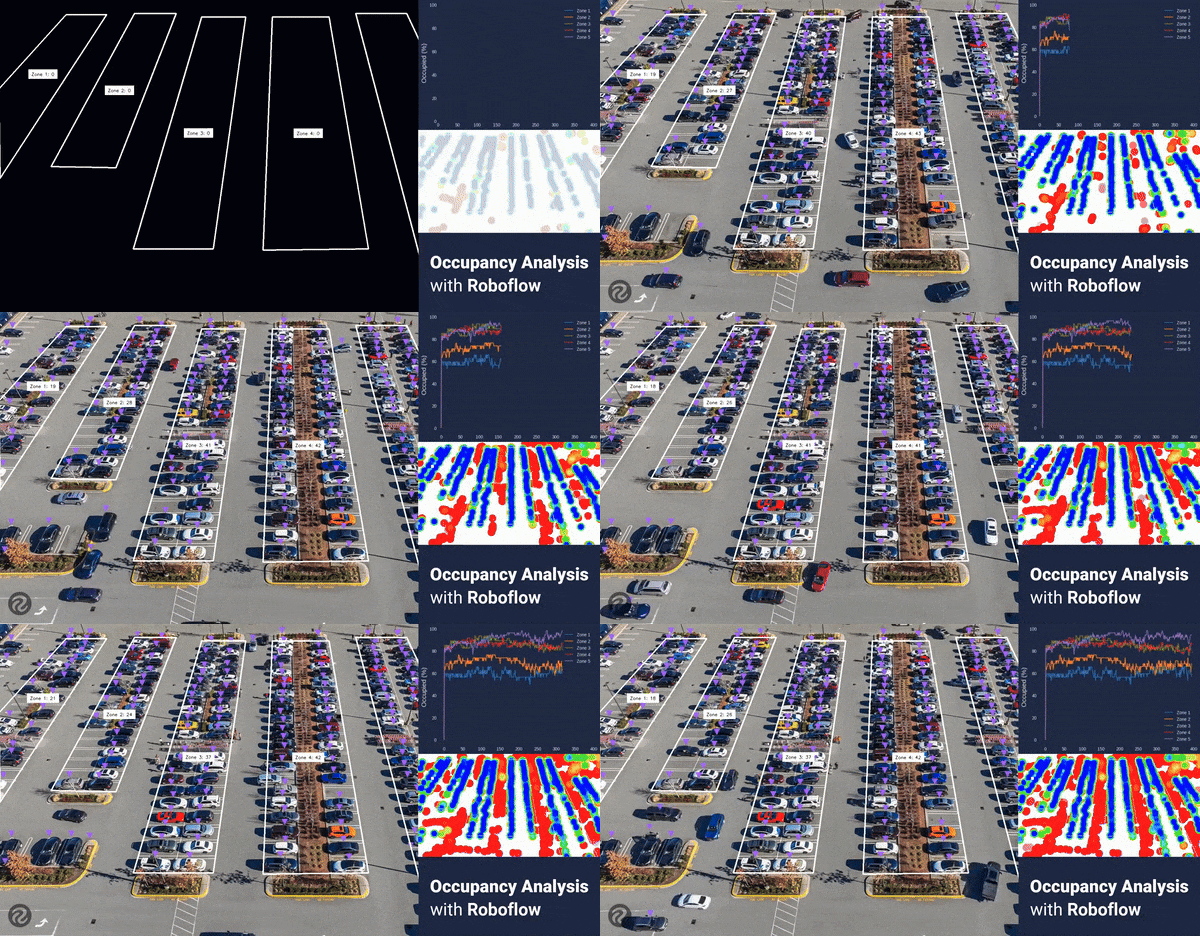
In this notebook, we will cover the following:

1. Getting training data
2. Training a object detection model
3. Detect vehicles
4. Analyze data and generate statistics

Before You Start

Let's make sure that we have access to GPU. We can use nvidia-smi command to do that. In case of any problems navigate to Edit -> Notebook settings -> Hardware accelerator, set it to GPU, and then click Save.

In [ ]:

!nvidia-smi

Install Relevant Packages

Here, we will install the Roboflow package, for uploading and training our model, and Supervision for visualization and extracting metrics from our predicted model results.

In [ ]:

!pip install roboflow supervision -q

Getting Video Data

We will start with turning a single video into a folder of frame images, for training our model. Upload your video and set your video's file path here.

In [ ]:

VIDEO_PATH = "/content/parkinglot1080.mov"

First, let's create a directory to save the video frames

In [ ]:

import os

FRAMES_DIR = "/content/frames"
os.mkdir(FRAMES_DIR)

Then, we can use Supervision's get_video_frames_generator function to get, then save, our video frames

In [ ]:

import supervision as sv
from PIL import Image

frames_generator = sv.get_video_frames_generator(VIDEO_PATH)

for i, frame in enumerate(frames_generator):
  img = Image.fromarray(frame)
  img.save(f"{FRAMES_DIR}/{i}.jpg")

print(f"Saved frames to {FRAMES_DIR}")

Saved frames to /content/frames

Random Crop Sampling (If Using SAHI)

If we are using SAHI (which we are in our example), randomly sampling cropped portions of our image can help mimic the effect of SAHI detection during training, improving performance.

In [ ]:

# Note: This code block was written by ChatGPT

import os
import random
from PIL import Image
import numpy as np

# import shutil
# shutil.rmtree("augmented")

def random_crop(img):
    width, height = img.size

    crop_width = random.randint(int(width * 0.1), int(width * 0.4))
    crop_height = random.randint(int(height * 0.1), int(height * 0.4))

    left = random.randint(0, width - crop_width)
    top = random.randint(0, height - crop_height)

    return img.crop((left, top, left + crop_width, top + crop_height))

def augment_images(source_folder, target_folder, num_images=100):
    if not os.path.exists(target_folder):
        os.makedirs(target_folder)

    all_images = [file for file in os.listdir(source_folder) if file.endswith('.jpg')]

    selected_images = np.random.choice(all_images, size=min(num_images, len(all_images)), replace=False)

    for i, filename in enumerate(selected_images):
        with Image.open(os.path.join(source_folder, filename)) as img:
            cropped_img = random_crop(img)
            cropped_img.save(os.path.join(target_folder, f'augmented_{i}.jpg'))

# Paths to the source and target folders
source_folder = '/content/frames'
target_folder = '/content/augmented'

# Augment images
augment_images(source_folder, target_folder)

Training a Model

Now that we have our images, we can upload our extracted frames as training data to Roboflow.

Upload Training Data

In [ ]:

# Upload the extracted frames to Roboflow
import os
import roboflow

rf = roboflow.Roboflow(api_key="YOUR_ROBOFLOW_API_KEY")
project = rf.workspace().project("parking-lot-occupancy-detection-eoaek")

for filename in os.listdir(FRAMES_DIR):
  img_path = os.path.join(FRAMES_DIR, filename)
  if os.path.isfile(img_path):
      project.upload(image_path=img_path)

loading Roboflow workspace...
loading Roboflow project...

Training Model Using Autodistill (Optional)

We can train our model using Automated Labeling, powered by Autodistill, to automatically label our data. Copy the code required for this section from the Roboflow app.

Note: It's not required to use Autodistill

In [ ]:

# PASTE CODE FROM ROBOFLOW HERE

Vehicle Detection

Now, we can run our model to get inference data for our video data.

Setup Model

First, set the model up as a callback function so that we can call it later on while using Supervision.

In [ ]:

from roboflow import Roboflow
import supervision as sv
import numpy as np
import cv2

rf = Roboflow(api_key="YOUR_ROBOFLOW_API_KEY") # Get your own API key - This one won't work
project = rf.workspace().project("parking-lot-occupancy-detection-eoaek")
model = project.version("5").model

def callback(x: np.ndarray) -> sv.Detections:
    result = model.predict(x, confidence=25, overlap=30).json()
    return sv.Detections.from_inference(result)

loading Roboflow workspace...
loading Roboflow project...

Configure Zones

Next, we will set up a list of the zones to be used with PolygonZone. You can get these polygon coordinates using this web utility.

For our example, we have have zones, but you can add as many or as little zones as you would like.

In [ ]:

# Polygons From PolygonZone

zones = [
    {
        'name': "Zone 1",
        'polygon': np.array([[229, 50],[-3, 306],[1, 614],[369, 50]]),
        'max': 32
    },
    {
        'name': 'Zone 2',
        'polygon': np.array([[465, 46],[177, 574],[401, 578],[609, 46]]),
        'max': 38
    },
    {
        'name': 'Zone 3',
        'polygon': np.array([[697, 58],[461, 858],[737, 858],[849, 58]]),
        'max': 46
    },
    {
        'name': 'Zone 4',
        'polygon': np.array([[941, 58],[909, 862],[1273, 858],[1137, 58]]),
        'max': 48
    },
    {
        'name': 'Zone 5',
        'polygon': np.array([[1229, 46],[1501, 1078],[1889, 1078],[1405, 46]]),
        'max': 52
    }
]

Setup Supervision

For our use case, we will use the following features of Supervision. Refer to the linked documentation for more details:

• ByteTrack: To track the location of our vehicles, so we can assess how long they are parked
• InferenceSlicer: A helper utility to run SAHI on our model
• TriangleAnnotator: To help visualize the locations of the vehicles
• HeatMapAnnotator: To generate heatmaps so we can identify our busiest areas
• PolygonZone, PolygonZoneAnnotator: To help count and identify vehicles in our respective zones and the annotator to help visualize those zones.

In [ ]:

tracker = sv.ByteTrack()
slicer = sv.InferenceSlicer(
    callback=callback,
    slice_wh=(800, 800),
    overlap_ratio_wh=(0.2, 0.2),
    thread_workers=10,
    iou_threshold=0.2
)
triangle_annotator = sv.TriangleAnnotator(
    base=20,
    height=20
)
heat_map_annotator = sv.HeatMapAnnotator()

def setup_zones(frame_wh):
  if zones:
    for zone in zones:
      zone['history'] = []
      zone['PolygonZone'] = sv.PolygonZone(
          polygon=zone['polygon'],
          frame_resolution_wh=frame_wh
      )
      zone['PolygonZoneAnnotator'] = sv.PolygonZoneAnnotator(
        zone=zone['PolygonZone'],
        color=sv.Color.WHITE,
        thickness=4,
    )

def process_frame(frame,heatmap=None):
    detections = slicer(image=frame)
    detections = tracker.update_with_detections(detections)

    annotated_frame = frame.copy()

    annotated_frame = triangle_annotator.annotate(
        scene=annotated_frame,
        detections=detections
    )

    if heatmap is None:
      heatmap = np.full(frame.shape, 255, dtype=np.uint8)

    heat_map_annotator.annotate(
      scene=heatmap,
      detections=detections
    )

    if zones:
      for zone in zones:
        zone_presence = zone['PolygonZone'].trigger(detections)
        zone_present_idxs = [idx for idx, present in enumerate(zone_presence) if present]
        zone_present = detections[zone_present_idxs]

        zone_count = len(zone_present)
        zone['history'].append(zone_count)


        annotated_frame = zone['PolygonZoneAnnotator'].annotate(
            scene=annotated_frame,
            label=f"{zone['name']}: {zone_count}"
        )

        # Heatmap
        heatmap = zone['PolygonZoneAnnotator'].annotate(
            scene=heatmap,
            label=" "
        )

    return annotated_frame, heatmap

Try With a Single Image

In [ ]:

image = cv2.imread("./frames/5.jpg")
image_wh = (image.shape[1],image.shape[0])
setup_zones(image_wh)

annotated_image, heatmap = process_frame(image)

sv.plot_image(annotated_image)
sv.plot_image(heatmap)

(1920, 1080)

Setup Graphs

Before we run the model on the entire video, we will set up the logic to generate our graphs using matplotlib.

In [ ]:

# Credit to https://matplotlib.org/matplotblog/posts/matplotlib-cyberpunk-style/ for graph styles
%matplotlib agg
import pandas as pd
import matplotlib.pyplot as plt
from PIL import Image
from io import BytesIO

def generate_graphs(max_frames):
  plt.ioff()
  # Plot Styles
  plt.style.use("seaborn-dark")
  for param in ['figure.facecolor', 'axes.facecolor', 'savefig.facecolor']:
      plt.rcParams[param] = '#212946'

  for param in ['text.color', 'axes.labelcolor', 'xtick.color', 'ytick.color']:
      plt.rcParams[param] = '0.9'


  dataframe = pd.DataFrame()
  graphs = {}


  for zone in zones:
    percentage_history = [(count/zone['max'])*100 for count in zone['history']]
    dataframe[zone['name']] = percentage_history
    plt.title(f'{zone["name"]} Usage')

    # Extra Styles
    fig, ax1 = plt.subplots()
    ax1.grid(color='#2A3459')

    # Data
    ax1.plot(zone["history"])

    # Axis Labeling
    plt.ylabel('Vehicles')
    plt.ylim(top=zone["max"])
    plt.xlim(right=max_frames)
    ax2 = ax1.twinx()
    ax2.set_ylabel('Occupied Percentage (%)')

    # Export Graph Image
    buf = BytesIO()
    fig.savefig(buf, format='png', bbox_inches='tight', pad_inches=0)
    buf.seek(0)
    graphs[zone['name']] = Image.open(buf)
    plt.close(fig)


  plt.ioff()
  dataframe.plot()

  # Axis
  plt.ylabel('Occupied (%)', fontsize=15)
  plt.ylim(top=100)
  plt.xlim(right=max_frames)

  # Export combined
  buf = BytesIO()
  plt.savefig(buf, format='png', bbox_inches='tight')
  buf.seek(0)

  plt.close()

  graphs['combined_percentage'] = Image.open(buf)

  return graphs

In [ ]:

generate_graphs(400)['combined_percentage']

Process Video

Now, we can process the video to get detections from the entire video.

In [ ]:

VIDEO_PATH = "/content/parkinglot1080.mov"
MAIN_OUTPUT_PATH = "/content/parkinglot_annotated.mp4"
frames_generator = sv.get_video_frames_generator(source_path=VIDEO_PATH)
video_info = sv.VideoInfo.from_video_path(video_path=VIDEO_PATH)

setup_zones(video_info.resolution_wh)


with sv.VideoSink(target_path=MAIN_OUTPUT_PATH, video_info=video_info) as sink:
  heatmap = None
  for i, frame in enumerate(frames_generator):
    print(f"Processing frame {i}")

    # Infer
    annotated_frame, heatmap = process_frame(frame, heatmap)

    # Save the latest heatmap
    Image.fromarray(heatmap).save(f"/content/heatmap/{i}.jpg")

    # Create Graphs
    graphs = generate_graphs(video_info.total_frames)
    graph = graphs["combined_percentage"].convert("RGB")
    graph.save(f"/content/graphs/{i}.jpg")

    # sv.plot_image(annotated_frame)

    # Send as frame to video
    sink.write_frame(frame=annotated_frame)

Processing frame 0

Processing frame 1

Processing frame 2

Processing frame 3

Processing frame 4

Processing frame 5

Processing frame 6

Processing frame 7

Processing frame 8

Processing frame 9

Processing frame 10

...

Generate Graphs/Heatmap Video (optional)

In [ ]:

import cv2
def create_videos_from_dir(dir,output):
  images = len(os.listdir(dir))-1

  sample_img_path = os.path.join(dir,f"1.jpg")
  sample_img = cv2.imread(sample_img_path)
  height, width, channels = sample_img.shape
  video_info = sv.VideoInfo(width=width,height=height,fps=24,total_frames=images)

  with sv.VideoSink(target_path=output, video_info=video_info) as sink:
    for i in range(images):
      path = os.path.join(dir,f"{i}.jpg")
      img = cv2.imread(path)
      sink.write_frame(frame=img)

# Graphs
create_videos_from_dir("/content/graphs","/content/parkinglot_graph.mp4")

# Heatmap
create_videos_from_dir("/content/heatmap","/content/parkinglot_heatmap.mp4")

Analyze Data

Lastly, we can analyze the data we got to extract quantitative metrics from our video.

Save your data for later

Using Pickle, we can save our zone detection data so that we can load it in for later analysis. Remember to download your file from the Colab file manager.

In [ ]:

import pickle

with open('parkinglot_zonedata.pkl', 'wb') as outp:
  pickle.dump(zones, outp, pickle.HIGHEST_PROTOCOL)

Import your data

To load your data back in, upload the saved file to the Colab environment and run the code cell.

In [ ]:

with open('parkinglot_zonedata.pkl', 'rb') as inp:
    zones_imported = pickle.load(inp)
    zones = zones_imported

Occupancy Per Section

Since we recorded the number of objects (vehicles) in each zone, we can compare that against our hardcoded max that we put in while setting up our zones. Using this data, we can calculate the average and median occupancy, as well as any other metrics such as the max or the minimum occupancy throughout that time period.

In [ ]:

import statistics
for zone in zones:
    occupancy_percent_history = [(count/zone['max'])*100 for count in zone['history']]
    average_occupancy = round(statistics.mean(occupancy_percent_history))
    median_occupancy = round(statistics.median(occupancy_percent_history))
    highest_occupancy = round(max(occupancy_percent_history))
    lowest_occupancy = round(min(occupancy_percent_history))
    print(f"{zone['name']} had an average occupancy of {average_occupancy}% with a median occupancy of {median_occupancy}%.")

Zone 1 had an average occupancy of 60% with a median occupancy of 59%.
Zone 2 had an average occupancy of 69% with a median occupancy of 68%.
Zone 3 had an average occupancy of 85% with a median occupancy of 85%.
Zone 4 had an average occupancy of 85% with a median occupancy of 85%.
Zone 5 had an average occupancy of 91% with a median occupancy of 92%.

Total Occupancy

Using the occupancy for the zones, we can also add up all the occupancy metrics throughout all the zones in order to calculate metrics for the whole parking lot.

In [ ]:

lot_history = []
for zone in zones:
    for idx, entry in enumerate(zone['history']):
      if(idx >= len(lot_history) or len(lot_history)==0): lot_history.append([])
      lot_history[idx].append(zone['history'][idx]/zone['max'])

lot_occupancy_history = [sum(entry)/len(entry)*100 for entry in lot_history]

average_occupancy = round(statistics.mean(lot_occupancy_history))
median_occupancy = round(statistics.median(lot_occupancy_history))
highest_occupancy = round(max(lot_occupancy_history))
lowest_occupancy = round(min(lot_occupancy_history))

print(f"The entire lot had an average occupancy of {average_occupancy}% with a median occupancy of {median_occupancy}%.")

The entire lot had an average occupancy of 78% with a median occupancy of 78%.

In [ ]:

print(lot_occupancy_history)

# [
#    ...
#    73.51691310215338,
#    73.34063105087132,
#    73.86694684034501,
#    ...
# ]

[0.0, 73.6265622249604, 73.51691310215338, 73.34063105087132, 73.86694684034501, 73.81677961626474, 74.2515622249604, 74.55142873907177, 74.34309540573842, 76.10547585518981, 75.33624508595904, 75.19454468110075, 74.56954468110075, 74.2334462829314, 74.07528017367835, 74.29457841929236, 74.08624508595905, 74.95162970134366, 75.19619491873496, 75.78914363668368, 76.15564307927008, 75.53779410901838, 75.6293272897964, 75.43910989849205, 76.54025846388546, 76.54025846388546, 77.77632312386316, 76.71654051516751, 77.70969019538813, 78.09430558000352, 77.13320718183418, 78.25247168925658, 79.48853634923428, 78.42875374053864, 78.28452297130787, 77.51782256644957, 78.28452297130787, 77.65952297130787, 78.60250542744822, 79.33715455025524, 79.33715455025524, 78.81083876078155, 78.66913835592325, 78.57045414539694, 78.04413835592325, 77.70803995775391, 77.60935574722761, 77.08303995775391, 77.70803995775391, 77.20662442058324, 78.11755559467231, 77.20662442058324, 77.20662442058324, 78.02602241389427, 77.20662442058324, 77.20662442058324, 78.21623980519861, 77.20662442058324, 76.53860822625124, 76.68030863110955, 76.92069324649417, 77.81768908056092, 76.68030863110955, 79.78422226133897, 79.01752185648066, 78.7315906823916, 79.25790647186528, 78.7315906823916, 78.1065906823916, 77.79957313853194, 77.08303995775391, 76.90675790647185, 77.64140702927888, 77.94842457313852, 77.2707269846858, 78.92345831133017, 78.5067916446635, 76.77811271489762, 78.07365927360208, 78.42622337616618, 79.27767265152849, 79.61212081206361, 81.54146863815058, 81.01515284867688, 80.1472378689198, 80.7541219268908, 79.0098574194684, 80.16117320894209, 79.74450654227543, 78.78340814410608, 79.88873731150619, 80.01947280408379, 80.35392096461891, 79.69851992020185, 79.31390453558646, 79.69851992020185, 80.08313530481722, 80.32351992020186, 79.69851992020185, 79.66646863815056, 80.49980197148389, 79.8706213694772, 78.86100598486182, 78.68725429795222, 80.46357008742592, 78.49703690664789, 78.35280613741712, 80.70813530481722, 80.27335269612156, 79.23168602945492, 79.5041219268908, 79.55681951534353, 79.50665229126326, 79.6163014140703, 81.9855659214927, 81.41073314557296, 82.03573314557296, 81.45671976764653, 81.3651865868685, 80.03043771636449, 81.374501261515, 81.40908290793874, 81.64946752332337, 82.17578331279704, 83.04534853018835, 82.17578331279704, 81.84386551663441, 80.88276711846505, 82.12979669072347, 80.46775068943262, 81.17034853018833, 80.75368186352169, 79.51761720354398, 81.18428387021063, 80.55928387021063, 79.7259505368773, 79.91616792818166, 80.35095053687732, 79.77446752332335, 79.79258346535234, 79.82463474740362, 80.01485213870797, 79.77446752332335, 79.3578008566567, 78.55651880537464, 78.58857008742592, 79.38985213870797, 79.38985213870797, 78.97318547204131, 78.41481840051634, 78.721835944376, 79.14946752332335, 79.3578008566567, 80.15908290793874, 79.59818547204131, 80.63985213870797, 81.47318547204131, 80.01485213870797, 81.61741624127208, 81.20074957460541, 80.99241624127208, 81.02446752332335, 81.40908290793874, 82.03408290793874, 81.64946752332337, 81.02446752332335, 81.02446752332335, 81.40908290793874, 80.36741624127208, 80.77014756791645, 80.86883177844277, 80.24383177844277, 81.01053218330107, 79.474601009212, 80.48421639382738, 80.85071583641377, 79.7103649592208, 80.52558235052514, 79.99926656105146, 80.85071583641377, 79.26461743824443, 79.16593322771813, 78.36465117643607, 78.78131784310274, 78.78131784310274, 79.19798450976941, 79.74241624127207, 81.20074957460541, 79.93263363257641, 79.38820190107376, 79.88961743824443, 79.67413307516283, 79.56448395235581, 79.14781728568914, 78.63246640849616, 78.2157997418295, 78.74926656105147, 78.36465117643607, 78.78131784310274, 79.16593322771813, 78.9575998943848, 79.5825998943848, 78.22295077157777, 78.73115061902247, 78.62150149621544, 78.1867188875198, 77.77005222085313, 78.20483482954879, 78.1727835474975, 77.78816816288212, 78.09518570674176, 78.20483482954879, 77.71057032212639, 79.0562841049111, 78.62150149621544, 80.52558235052514, 79.47295077157777, 78.11330164877074, 78.28958370005282, 78.00365252596374, 77.20237047468169, 78.20483482954879, 77.58698585929707, 77.58698585929707, 77.6785190400751, 77.6785190400751, 78.58945021416417, 77.61188611160007, 78.12723698879304, 75.51758786598603, 75.08280525729039, 78.24403714134836, 76.3234905826439, 77.37612216159127, 77.23442175673296, 77.76073754620666, 78.30516927770933, 76.52467288622894, 76.03040837880654, 76.04852432083553, 76.86792231414657, 75.85665669189696, 75.90517367834302, 77.24373643137945, 77.00797248137064, 78.44521944493339, 77.77467288622894, 76.7148902775333, 77.53428827084431, 77.72450566214869, 76.1885744880596, 75.53152320600833, 76.01229243677756, 74.26802792935516, 74.34309540573842, 76.700954937511, 75.29575925599954, 74.87194155958458, 75.94565950830253, 75.32065950830254, 75.16249339904945, 75.91360822625126, 75.88155694419997, 77.14967288622894, 77.29137329108724, 76.56603884292672, 75.07609429091121, 76.80642345831133, 76.38975679164466, 77.09950566214869, 77.90078771343074, 77.0674543800974, 76.10635598192805, 77.74515196855015, 78.58945021416417, 78.74761632341725, 77.83668514932818, 77.66205333568033, 78.97153523440709, 76.8426553423693, 77.11762160417767, 76.73300621956228, 76.90928827084433, 78.01758786598603, 77.28972305345303, 76.36485653934166, 77.6924543800974, 78.63543683623774, 77.41748811828903, 76.78152320600834, 75.35524115472627, 77.16360822625126, 77.07207504547323, 75.98024115472629, 76.49559203191927, 75.64414275655695, 76.35389162706097, 75.19542480783899, 76.36485653934166, 76.46354074986797, 77.97838555418647, 77.71057032212639, 78.07706976471279, 77.11597136654345, 78.60338555418647, 78.50470134366016, 79.03816816288212, 80.36576600363784, 76.60777151909876, 77.54360294549082, 76.63267177140176, 79.22838555418647, 77.97838555418647, 78.27146775802383, 80.78243267030452, 76.76593762835181, 78.57430469987679, 78.1757539752391, 77.35635598192806, 77.35635598192806, 78.74508595904477, 77.8341547849557, 78.86188611160007, 76.89117232881536, 77.55918852314733, 78.36762160417766, 77.19818987267499, 77.63297248137064, 77.63297248137064, 76.43992401572494, 76.92322361086663, 77.43142345831131, 76.48844100217099, 75.82207504547321, 79.310604060318, 79.310604060318, 78.78428827084433, 79.2119198497917, 77.63297248137064, 78.25082145162237, 79.07021944493339, 79.07021944493339, 78.21877016957109, 76.34674059731267, 77.84130581470399, 77.25767177140176, 78.02437217626006, 77.49805638678637, 76.48844100217099, 77.06327377809072, 77.06327377809072, 78.9534192923781, 78.3284192923781, 78.12008595904476, 77.49508595904476, 77.33691984979171, 77.67136801032682, 77.26863668368246, 76.71907087953998, 77.22727072698468, 77.12693627882416, 74.78972305345305, 76.03972305345303, 76.71026961215748, 75.5589538226838, 75.65510766883764, 76.08273924778501, 77.04933843806842, 75.62305638678637, 77.04933843806842, 77.5756542275421, 76.56603884292672, 77.2091547849557, 75.52437217626006, 76.98270550959337, 77.74940591445169, 77.99232089420876, 77.60770550959337, 78.42710350290443, 78.04248811828904, 78.3174543800974, 77.17710350290442, 76.68283899548202, 76.5841547849557, 76.5951196972364, 75.27049228422226, 74.43297834888224, 74.86776095757789, 74.51057618963797, 77.22727072698468, 76.21600510473507, 77.48412104676406, 76.84815613448336, 77.04933843806842, 76.9506542275421, 77.99232089420876, 76.98270550959337, 75.52734260400165, 75.8132737780907, 77.93962330575603, 76.74529132195038]

In [ ]:

%matplotlib inline

import matplotlib.pyplot as plt

fig, ax1 = plt.subplots()
plt.title('Total Lot Usage')
ax1.grid(color='#2A3459')

ax1.plot(lot_occupancy_history)
ax1.set_ylabel('Occupied Percentage (%)')

plt.ylim(top=100)
plt.xlim(right=len(lot_occupancy_history))

plt.show()

Busy Areas

Using Supervision's heat map annotator, we can use heatmaps while transforming the images in order to create images on top-down views of each zone.

In [ ]:

import cv2
import numpy as np

def transform_image(image, points):
    width = max(np.linalg.norm(points[0] - points[1]), np.linalg.norm(points[2] - points[3]))
    height = max(np.linalg.norm(points[0] - points[3]), np.linalg.norm(points[1] - points[2]))
    dest_points = np.array([[0, 0], [width - 1, 0], [width - 1, height - 1], [0, height - 1]], dtype="float32")
    matrix = cv2.getPerspectiveTransform(points.astype("float32"), dest_points)
    transformed_image = cv2.warpPerspective(image, matrix, (int(width), int(height)))

    return transformed_image

def generate_top_down_views(frame,show=True):
  heatmap = cv2.imread(f"heatmap/{frame}.jpg")
  image = cv2.imread(f"frames/{frame}.jpg")

  images = []

  for zone in zones:
    if show: print(f"Occupancy Visualization of {zone['name']}")
    top_down_image = transform_image(image, zone['polygon'])
    top_down_heatmap = transform_image(heatmap, zone['polygon'])

    combined_image = cv2.addWeighted(top_down_image, 0.7, top_down_heatmap, 0.3, 0)

    if show: sv.plot_image(combined_image, size=(5,5))

    images.append(combined_image)

  return images

In [ ]:

generate_top_down_views(400)

In [ ]:

import os
import numpy as np
from PIL import Image
import supervision as sv

for filename in os.listdir("frames"):
  img_path = os.path.join("frames", filename)
  heatmap_path = os.path.join("heatmap", filename)
  if os.path.isfile(img_path) and os.path.isfile(heatmap_path):
    frame = int(filename.replace(".jpg",""))
    images = generate_top_down_views(frame,False)
    gap = 10

    pil_images = [Image.fromarray(image) for image in images]

    # Resize images to have the same width
    widths, heights = zip(*(i.size for i in pil_images))
    max_width = max(widths)
    total_height = sum(heights) + gap * (len(images) - 1)
    resized_images = [i.resize((max_width, int(i.height * max_width / i.width))) for i in pil_images]

    # Create a new image with the correct combined size
    combined_image = Image.new('RGB', (max_width, total_height))

    # Paste each image into the combined image with the specified gap
    y_offset = 0
    for img in resized_images:
        combined_image.paste(img, (0, y_offset))
        y_offset += img.height + gap

    combined_image = combined_image.rotate(90, expand=True)

    combined_image.save(f"sectionheatmaps/{frame}.jpg")

    sv.plot_image(np.array(combined_image))